Zonal Statistics for OpenStreetMap in the browser
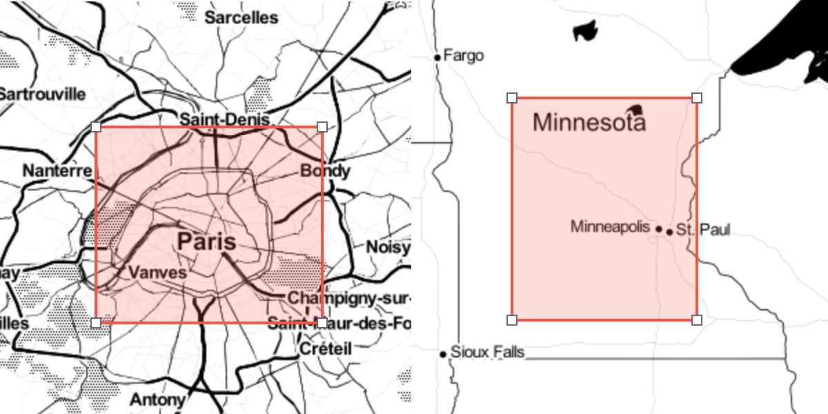
A common user interaction in GIS applications is selecting a bounding box or polygon:
Your application may then use this polygon to do things like:
Render a high resolution, printable map image.
Generate a report of the surface area of buildings.
Calculate an isochrone map of distance to transit.
Users of your service expect that any action will complete in a reasonable amount of time. It’s smart to build in a limit for the amount of data processed on the server. One simple way to do this is an area limit, for example: 100 square kilometers.
Using total area doesn’t work well for datasets of man-made objects like OpenStreetMap. The density of features has huge variance in different parts of the world. In the image above, the area on the left is only part of Paris and contains about 10 million nodes. The area on the right is most of the U.S. state of Minnesota, and also has about 10 million nodes. A system limit designed for the densest areas would be too restrictive.
Density
Instead of having an area limit, we can first test the area for the count of features, and then provide feedback in the UI if the limit is exceeded. Common ways to count are:
For data in PostgreSQL, query over a spatial index using a function like ST_Intersects, returning a row count.
For OpenStreetMap, use Overpass API to count nodes or features matching a tag, returning a count output.
This information can be exposed to a web browser via API.
Faster, Simpler
The previous approach has the major drawback of needing a remote, blocking server call. We can instead design a quicker way to estimate the number of features without a dynamic query. This allows for near-instant feedback in the UI, and less moving parts, at the cost of being a coarse approximation.
The GeoTIFF format is a natural fit for this problem. It’s readable by all GIS libraries, supports compression, and embeds a geographic projection.
Each pixel in this image is one level 12 Web Mercator Tile, and each sample is a 16 bit unsigned OpenStreetMap node count (in thousands). This is too dark to be visible to the human eye, but normalizing the color range results in this image:
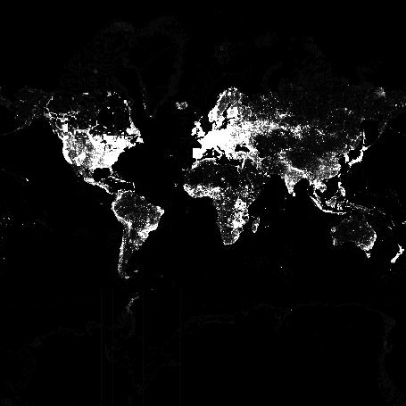
The resulting compressed GeoTIFF is only 212 KB, which is reasonable to deliver to web browsers. The source code for generating this GeoTIFF is available at github.com/protomaps/OSMEstimator.
Calculating Estimates
Any zonal statistics library can be used to compute the sum total of an area of interest over the GeoTIFF’s samples. The GeoBlaze library implements this in JavaScript. The Rasterio library implements this in Python. Example of computing a sum in Python:
import pyproj
from rasterio import mask
from shapely.geometry import shape

RASTER = rasterio.open('osm_nodes.tif')
PROJECT = partial(pyproj.transform,pyproj.Proj(init='epsg:4326'),pyproj.Proj(init='epsg:3857'))
transformed = transform(PROJECT,shape(geom)) #geom is a GeoJSON-like dict
masked = mask.mask(RASTER,[transformed],all_touched=False)
estimate = masked[0].sum() * 1000
Limitations
The choice of zoom level 12 and the accuracy of the estimation rely on query areas being significantly larger than the pixels of the GeoTIFF. Different applications may want to modify this code for:
Specific features: Modify the program to only consider ways tagged building=yes, instead of all OpenStreetMap nodes.
If the relevant area is only part of the world, the GeoTIFF size can be reduced by cropping the raster.
Trade-offs between estimation accuracy and file size can be controlled by using 8, 16 or 32 bit samples.